Being in Operations means putting either Excel or Google spreadsheets though its paces. The use cases are endless, budgets, forecasting, auditing, tracking, modelling, and so forth. So today I thought I would share with you some formula’s I have used and examples on where you might use these formulas. All the formulas I am suggestion worth in both Google Docs – Spreadsheets and Excel 2012 (or higher).

Useful Formulas

The CONCENTATE Function

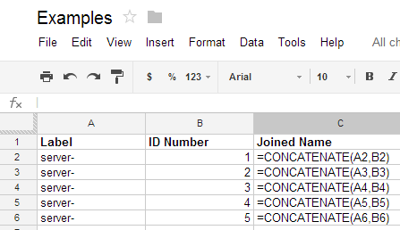
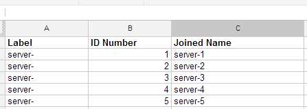
Useful for joining multiple columns of data together to form one word or merged result. For example, if I wanted to create a list of server labels for a labeling machine. Usually a server label has a name with a number, similar to server-1. So we create a column full of the text “server-“, then create another column with the ID number. We then put in the CONCENTATE formula similar to the below picture,

The end result looks like the following,

The REGEXMATCH Function

Often I come across situations where I have similar versions or similar logs for a large range of servers. I want to be able to quickly check for certain criteria on a large scale. So in my example, I have column A with the log outputs, and then column B is where my formula to check if the logs contained the word / text “blue”.

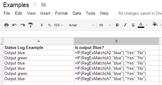
Combining the use of an IF statement and the RegExMatch formula. I am able to check if the text in a particular cell contains the text “blue”. If it does, flag the result as YES, if not, flag it NO. The end result is like this,

The NESTED REGEX MATCH Function

Building on the above example, there may be situations where you want to run multiple “checks” against a cell. So by this I mean the IF statement will check more than one criteria. A good use for this is trying to figure out how many IP Addresses are associated with certain IP Range allocations like /29 or /30. Often we have records showing servers have an IP Address range of 10.1.1.1/29 allocated, however this is not easy to quickly figure out how many IP’s that is, to then perform formula’s and calculations on. So the following use of nested RegExMatch functions can solve that problem. Essentially I have create an IF Statement within the first IF statement. So basically it checks the cell reference for the text “/28”. If that is there, it says that has 16. If /28 is not there, it checks for /29, and returns an 8. If neither option is there it returns a 0. See the following example,

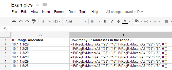
The end result would look like this,

The RANDBETWEEN Formula

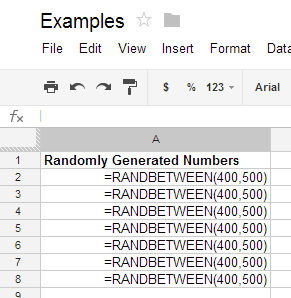
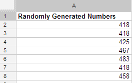
Not a big powerful formula, but it helps randomly generate numbers which is useful sometimes. So just as it sounds, you give the formula a bottom number and a top number, it will then choose a number randomly between that range.

The end result is,

I hope you find these all as useful as I did. If you do have any other useful formula’s worth noting, please leave a comment. I’d love to hear from you.